

OPAL 2.8/12 C | Datasheet
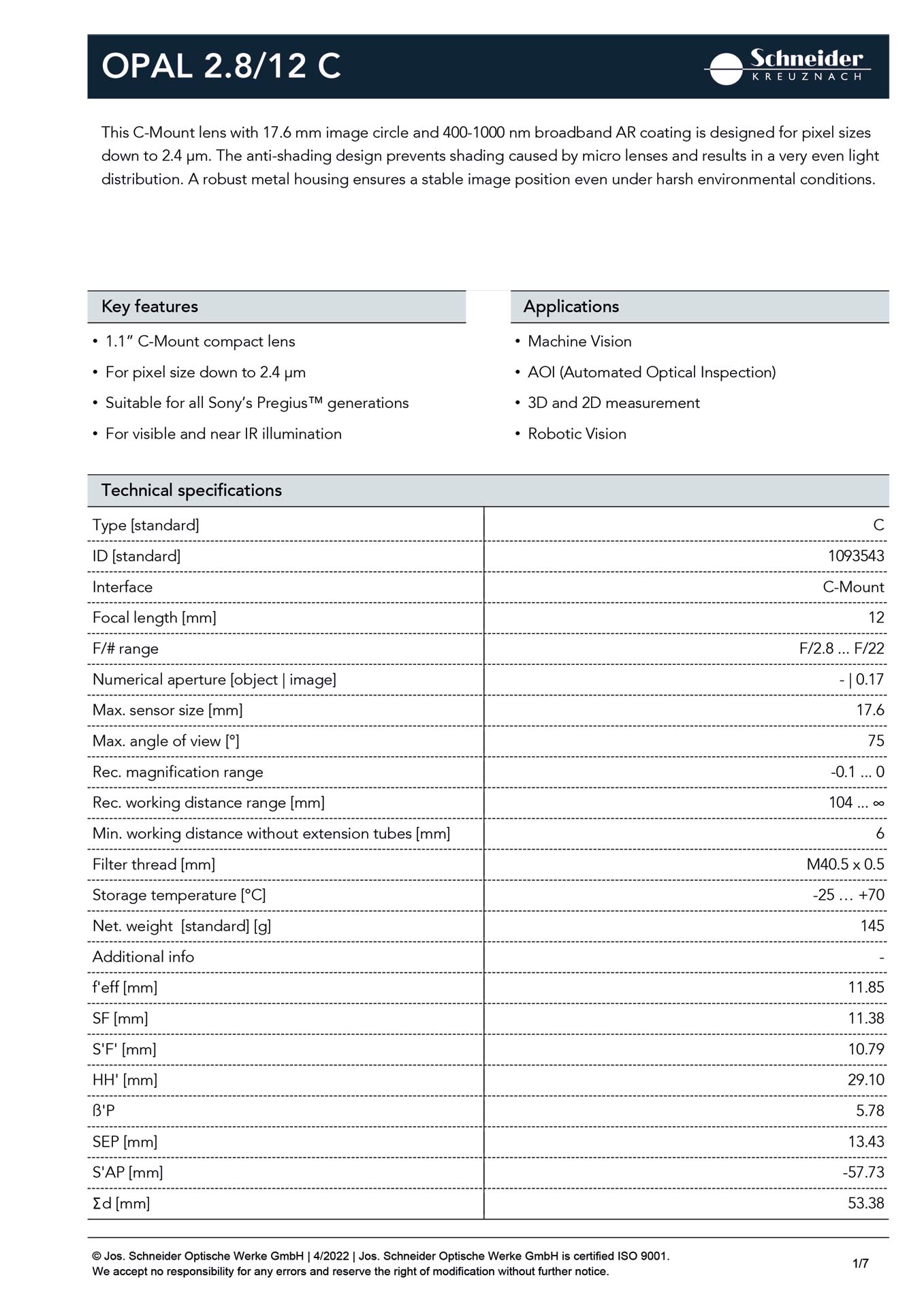
Mechanical dimensions, lens data, MTF
It is essential for our customers to understand how to effectively read and use lens specifications to make informed decisions in industrial imaging applications. Our guide offers a systematic approach to decoding key specifications found in lens data sheets. Learn how to interpret critical parameters. By mastering the skill of analyzing lens data sheets, you can confidently assess lenses to ensure they meet your specific requirements.
In the optical and mechanical PDF-data sheets you will find the following information:
Mechanical dimensions, lens data, MTF
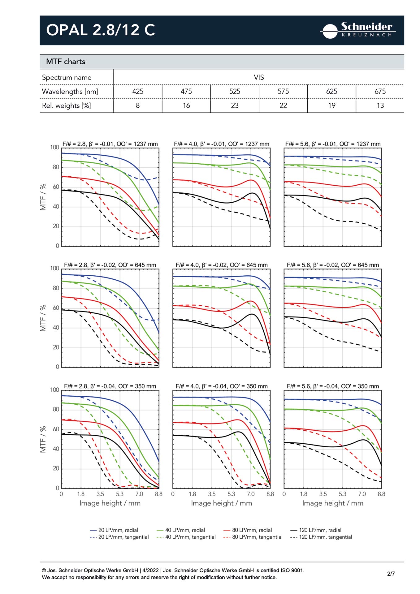
MTF chart
All images, from photographic lenses, vary in intensity from their center to the edge. This can be bad. Therefore it is necessary to examine the performance of a lens in this area, to determine its suitability (or lack of it) for a particular application. There are several factors involved: There is a natural decrease in illumination from center to edge of the image circle (less at the edge) which varies with the fourth power of the cosine of the field angle.
The cos4 w-law of relative illumination
The second major factor which has an impact upon uniformity of illumination is mechanical vignetting of the image. This simply means that some rays are blocked by mechanical parts, barrel walls etc. The effect of vignetting can be greatly reduced by using a smaller aperture. lt is therefore necessary to represent several apertures on graphic representations of illumination.
The term distortion refers to a change in the geometric representation of an object in the image plane. A rectangle might, for instance be reproduced with a pincushion, or barrel shape, if the distortion of the optical system is positive, or negative, respectively.
Distortion, barrel or pincushion, may also change with image height, distortion also changes with magnification. ln our data sheets, distortion is always represented in a manner which corresponds to the particular application. Enlarging lenses, for example, are represented showing the enlarger baseboard as the image plane.
Distortion
All optical materials transmit certain wavelengths with more, or less efficiency. Some wavelengths are reflected, or absorbed by these materials in different amounts. Lenses are, of course, manufactured from optical glass, which may be of many types and combinations. Each type of glass, and each type of surface coating, will show distinct spectral transmission characteristics. Therefore it is important, when evaluating a lens, to study the actual transmission data, which is furnished in our spectral transmission curves. While all Schneider-Kreuznach lenses are calculated and manufactured to produce excellent, color free images, you will notice subtle tendencies of a lens toward warm or cold rendition. You may also use this data for comparison to other lenses, this could, in some cases prevent the purchase of an inappropriate lens.
Spectral transmission as function of the wavelength
Let us assume an ideal lens and a photographic scene which is composed of many different coarse and fine structures, e. g. a distribution of broad and fine line elements of intensity variations. ln this situation, the hypothetical, ideal lens will produce an image which reproduces the object faithfully. More precisely, this means that the spatial variation of density in the image is an exact representation of the intensity modulation in the object, regardless of the width of the lines.
We have been discussing an ideal situation, which, for physical reasons, cannot be realized. ln reality, coarse lines can be reproduced more easily than fine lines, and coarse lines can be reproduced with a higher modulation (contrast) than fine lines. We refer to this spatial variation (coarse and fine) by the number of line pairs per millimeter, either at the subject, or the image.
Modulation Transfer function (MTF) compares the remaining modulation in the image plane with the original object. The result is expressed in percent, as a function of spatial frequency (lp/mm), see figure on the right.
Explanation of the MTF
lt is apparent that the modulation transfer decreases when the spatial frequency increases. At some point, as the spatial frequency increases, the modulation will be zero. The modulation transfer function of the lens should be high over the entire region of spatial frequencies which is to be considered. The upper Limit, of spatial frequency, for a particular application is dependent upon the particular constellation of factors such as film/CCD formal size, film/CCD type, lens aperture, and desired performance.
A single MTF graph, done in the customary fashion, is representative of a small image area which could be anywhere within the image, but typically is done on axis, and at intervals up to the image diagonal. To evaluate the performance of a lens over its entire image circle, one would have to examine a large number of MTF graphs.
Consequently, we often use another method of graphic representation for MTF. This method shows the modulation transfer as a function of image height, for a few meaningful spatial frequencies. Because it is relatively easy to evaluate the overall image performance of a lens, when viewing this type of graph, Schneider-Kreuznach uses this method of representation in it's data sheets.
Of course, it couldn't be quite as simple as that; a further characteristic of the imaging process is the fact that a beam of rays emerging from a lens, exhibits differing properties, dependent on its incidence angles. What this means, in a very practical way, is that object patterns with different orientations for example perpendicular to each other, will reproduce differently.
Therefore, it is necessary to select more than one orientation of the test pattern used in evaluation, to be sure of an accurate evaluation of the lens. Under normal circumstances, it will be sufficient to select two mutually perpendicular Orientations of line elements, as illustrated in the figure on the right.
There will therefore be two different sets of MTF data representing radial and tangential orientation of test patterns. ln our diagrams, the MTF for the tangential orientation will be shown in dashed lines.

lt is possible to use a lens in a variety of ways, and this can affect the performance of the lens, as represented by the MTF data. ln particular the image magnification, and aperture at which the lens is used, have a large effect on the performance of a lens.
For a particular optical system, there is always a theoretical limit to performance. This limit also depends on the field angle which is important for wide angle systems. Generally there will be a decrease in MTF values with the cosine of the field angle (for the radial orientation) and with the third power of cosine of the field angle for tangential orientation.
The figure on the left gives an example of a diffraction limited (perfect) optical system for 20 lp/mm at f-22, as a function of field angle.
Please do not hesitate to contact us if you have any questions. Our dedicated team is here to help you every step of the way.
Whether you need assistance with product selection, technical specifications, or general inquiries.
Jos. Schneider Optische Werke GmbH
Ringstraße 132
55543 Bad Kreuznach | Germany
Tel: +49 (0) 671 601 205
isales(at)schneiderkreuznach.com
Contact form